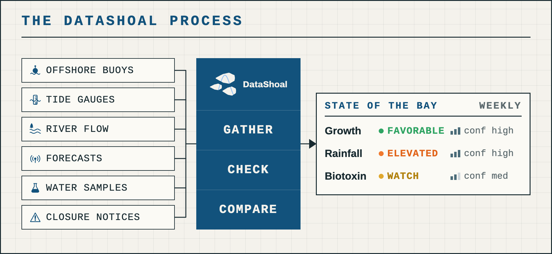
For the first post in our new weekly series, we are going to walk through the DataShoal process in more detail than the About page or the introduction post. Going forward, we’ll cover a new topic every few weeks and break it down one post at a time. Next week opens the first of those topics: what the current El Niño might mean for West Coast shellfish aquaculture. Each week we will state a hypothesis, look at what the published literature suggests, and see what current climate, oceanographic, and environmental data can add.
The first breakdown in that El Niño series is rainfall: what past El Niño winters can tell us about this one, how much of an increase over an average year to expect, and how the effect differs along the coast. From there we will move to the California Current and sea surface temperature (SST), and what those shifts could mean for phytoplankton communities and the potential for harmful algal blooms.
This week, though, is back to basics: how DataShoal approaches the problems underneath all of that. An offshore buoy, a pier-mounted sensor, and a weekly phytoplankton sample have to be brought onto the same playing field before anyone can assess conditions across a bay. Those readings then have to be turned into an assessment of what they mean for shellfish farmers, in a way that is accurate and repeatable. And AI models have to be put to work exploring complex relationships while staying grounded in documented facts. The graphic above is the short version: gather, check, compare.
Gather
The DataShoal process begins by gathering data from a wide range of public sources. I’d like to take this opportunity to thank the hardworking folks at CeNCOOS, SCCOOS, NOAA, USGS, and the many other government and academic groups who do the fundamental work of deploying sensors, maintaining them, and making the data available in a reliable and readable form. It is easy to forget that behind the rows and columns of a spreadsheet is a team of scientists and technicians hauling sensors and probes in and out of the water for routine cleaning, maintenance, and troubleshooting. Everything downstream depends on clean sensors and clean data. For more on the datasets we use, head to the map on any of the bay pages. Click a station marker and the pop-up shows what it measures, why it matters, who operates it, and how often it updates, with a Source link at the bottom that opens the provider’s page for more detail or for downloading the data for your own investigations. The full source list is in Many sources, one standard.
Check
Once we’ve identified the datasets we want, we have to get them all on the same page. A few of the factors we have to consider at this point:
- Differing units: a regulator’s temperature threshold written in Fahrenheit against sensors that report in Celsius, or a chlorophyll reading labelled micrograms per liter by one provider and milligrams per cubic meter by another (the same number, two labels).
- Parameter names: the same water temperature arrives as “sea surface temperature” from a NOAA buoy, “sea water temperature” from a CeNCOOS sensor, and plain “Temp” on a weekly sampling sheet. Two of those we deliberately never merge, because the offshore buoy and the in-bay sensor barely track each other, and averaging them would produce a number that describes neither.
- Cadence of readings: every six minutes for a tide gauge, roughly every ten for a buoy or in-bay sensor, every fifteen plus a daily mean for a river gauge, and about once a week for a phytoplankton sample.
- Idiosyncrasies of each dataset: a chlorophyll sensor that stops varying is more likely fouled than measuring a still bay, and a temperature of -9999 is a feed’s way of saying “no reading”, which averaged in by accident would drag a day’s mean below freezing.
One way we solve this is by holding every source to the same standard. DataShoal uses the QARTOD manuals (Quality Assurance / Quality Control of Real-Time Oceanographic Data), published by the U.S. Integrated Ocean Observing System (IOOS), as the benchmark, and runs them with the open-source test library the ocean-observing community maintains, pinned to one exact version. Where a provider ships its own quality flags, as NOAA’s tide gauges do, we keep them and layer QARTOD on top. Readings that fail are flagged and kept, never deleted or clipped, so the record shows both what was measured and what was doubted. The other way we handle such different sources is by taking a page from enterprise data engineering: instead of shoehorning everything into a single fixed database, we use a data lakehouse, which keeps the raw readings as they arrived, the checked readings with their flags, and the derived weekly indicators as three separate layers. Nothing in a later layer ever overwrites an earlier one.
Compare
So now we have a wide range of datasets, quality-controlled to the same standard and in the same place. The next step is turning those streams into meaningful signals for the conditions our shellfish crops actually experience, and doing it the same way every week. For that we borrow a practice from software engineering called “configuration as code”. Instead of a set variable here, a reference file there, and on-the-fly adjustments, we record everything in machine-readable definition files. These run from the version-stamped quality rules that judged each reading, through the temperature and salinity windows that define favorable growth for Pacific oysters, to the percentile cut at which river flow counts as elevated and the number of days after which a biotoxin sample is too old to rely on. Every one of those parameters has to cite a source in our reference library; a threshold with no citation does not get used. With so much uncertainty already present in the systems we study, the goal is never to add any of our own in the processing. The indicators DataShoal produces are a reproducible function of the checked data and that configuration: same inputs, same settings, same result, every time, and every report is stamped with the data run it was built from. If there is ever a question about an indicator, we can trace it back through the checked readings to the exact raw data that came in.
Where AI fits
The last piece is where AI models fit, and how we use them without throwing away the data checks and the repeatability above. The answer is the same practice again. In the weekly report, every number is computed by code before the model sees anything. The model’s only job is to write the narrative, and an automatic check then rejects any draft containing a number that is not in the computed results, or a status milder than the one computed. A rejected narrative is dropped, not published. In our investigations, like the El Niño series starting next week, the same idea holds. The analysis runs as scripts built on well-established Python libraries like pandas, NumPy, and SciPy, and every table and figure a script produces is written to disk with a fingerprint, so a re-run has to reproduce it byte for byte. Each step gets an adversarial review before anything downstream is allowed to use it. Casting that wide net first, well over a hundred tables and figures for a single question, means the model’s last-mile job is comparing needles we have already pulled and can trace back to the script that made them, not searching the haystack. The second facet is where the model’s knowledge comes from. Instead of relying on a black box of training data, we assemble a library of the relevant literature, in this case a bibliography of roughly two hundred papers built with OpenAlex, scored and narrowed to a core set that is read in full and catalogued so that every claim can cite the paper it came from. With our analysis outputs as the building blocks and the literature as the blueprint, the final assembly becomes a repeatable process, and the model is the tool best suited to fitting the pieces together in a structured way.